Vector Fields in Augmented Reality

The tube body is generated by creating rings of vertices along the length, then connecting them with triangles:

private generateSingleTube(gridX: number, gridY: number, pathLength: number, circleSegments: number): void {
    const startVertexIndex = this.meshBuilder.getVerticesCount();

    // Generate tube body vertices
    for (let i = 0; i < pathLength; i++) {
        const t = i / (pathLength - 1);

        for (let j = 0; j < circleSegments; j++) {
            const theta = (j / circleSegments) * Math.PI * 2;
            const localX = Math.cos(theta);
            const localY = Math.sin(theta);

            this.meshBuilder.appendVerticesInterleaved([
                0.0, 0.0, t,           // position: unused, unused, t
                0.0, 0.0, 1.0,         // normal: unused, unused, isTube=1
                localX, localY,        // texture0: unit circle coords
                gridX, gridY           // texture1: grid indices
            ]);
        }
    }

    // Generate indices for tube body
    for (let segment = 0; segment < pathLength - 1; segment++) {
        for (let i = 0; i < circleSegments; i++) {
            const current = startVertexIndex + segment * circleSegments + i;
            const next = startVertexIndex + segment * circleSegments + ((i + 1) % circleSegments);
            const currentNext = startVertexIndex + (segment + 1) * circleSegments + i;
            const nextNext = startVertexIndex + (segment + 1) * circleSegments + ((i + 1) % circleSegments);

            this.meshBuilder.appendIndices([
                current, next, currentNext,
                next, nextNext, currentNext
            ]);
        }
    }

    // Generate end caps for this tube
    this.generateSingleTubeCaps(gridX, gridY, startVertexIndex, pathLength, circleSegments);
}

The end caps are created by adding a center vertex and connecting it to the ring vertices in a fan pattern:

private generateSingleTubeCaps(gridX: number, gridY: number, startVertexIndex: number, pathLength: number, circleSegments: number): void {
    const tubeVertexCount = pathLength * circleSegments;

    // START CAP (at t = 0)
    const startCapIndex = this.meshBuilder.getVerticesCount();
    this.meshBuilder.appendVerticesInterleaved([
        0.0, 0.0, 0.0,         // position: unused, unused, t=0
        0.0, 0.0, 0.0,         // normal: unused, unused, isCap=0
        0.0, 0.0,              // texture0: center
        gridX, gridY           // texture1: grid indices
    ]);

    for (let i = 0; i < circleSegments; i++) {
        const current = startVertexIndex + i;
        const next = startVertexIndex + (i + 1) % circleSegments;
        this.meshBuilder.appendIndices([startCapIndex, next, current]);
    }

    // END CAP (at t = 1)
    const endCapIndex = this.meshBuilder.getVerticesCount();
    this.meshBuilder.appendVerticesInterleaved([
        0.0, 0.0, 1.0,         // position: unused, unused, t=1
        0.0, 0.0, 0.0,         // normal: unused, unused, isCap=0
        0.0, 0.0,              // texture0: center
        gridX, gridY           // texture1: grid indices
    ]);

    const lastRingStart = startVertexIndex + (pathLength - 1) * circleSegments;
    for (let i = 0; i < circleSegments; i++) {
        const current = lastRingStart + i;
        const next = lastRingStart + (i + 1) % circleSegments;
        this.meshBuilder.appendIndices([endCapIndex, current, next]);
    }
}

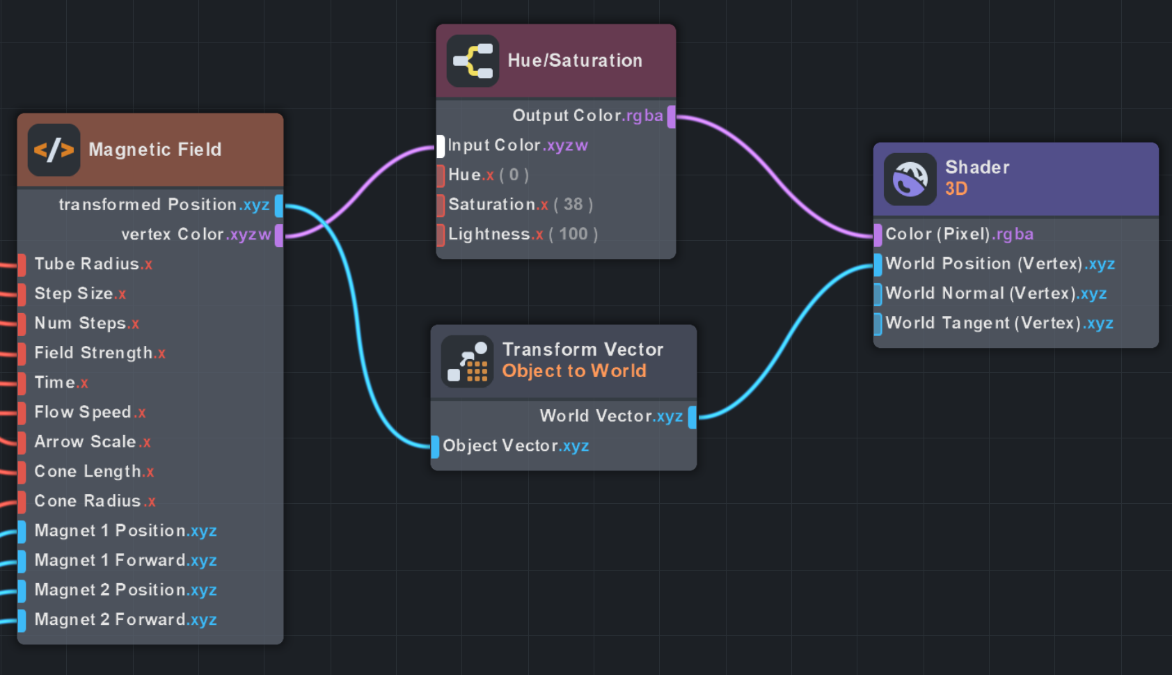
A key node from the material editor to make everything work is the Object to World converter. This transforms our computed vertex positions from object space into world space, ensuring the deformed tubes render correctly regardless of the object’s transform. Since you’re here, I might as well recommend you another node: Hue/Saturation. Lens Studio renders low value colors as transparent, so by using this node you can adjust the value color channel independently. It’s also useful for making colors pop by raising saturation.

Each dipole creates a vector field based on its magnetic moment $\mathbf{m}$ and the displacement $\mathbf{r}$ from the dipole:

$\mathbf{B}(\mathbf{r}) = \frac{3(\mathbf{m} \cdot \hat{\mathbf{r}})\hat{\mathbf{r}} - \mathbf{m}}{r^3}$

The field magnitude falls off as the inverse cube of distance: $|\mathbf{B}| \propto \frac{1}{r^3}$.

To trace flow lines through this field, we use Euler integration: starting from a sample point $\mathbf{p}_0$, we repeatedly query the field and step in its direction:

$\mathbf{p}_{n+1} = \mathbf{p}_n + \hat{\mathbf{B}}(\mathbf{p}_n) \cdot \Delta s$

where $\hat{\mathbf{B}}$ is the normalized field direction and $\Delta s$ is the step size. Combining two dipoles produces the characteristic looping field lines.

The dipole formula translates directly to GPU code:

vec3 dipoleMagneticField(vec3 point, vec3 dipolePos, vec3 moment) {
    vec3 r = point - dipolePos;
    float dist = length(r);

    if (dist < 0.1) {
        return moment * FieldStrength * 2.0;  // Inside dipole
    } else {
        vec3 rHat = r / dist;                           // r̂ = r/|r|
        float dist3 = dist * dist * dist;               // r³
        float mDotR = dot(moment, rHat);                // m · r̂
        vec3 B = (3.0 * mDotR * rHat - moment) / dist3; // B = (3(m·r̂)r̂ - m) / r³
        return B * FieldStrength;
    }
}

Euler integration runs in the vertex shader, stepping each vertex along the field:

for (int i = 0; i < 64; i++) {
    if (i >= clampedStepIndex) break;
    prevPos = pos;
    pos += getMagneticField(pos) * StepSize;  // p_{n+1} = p_n + B(p_n) · Δs
}

A separate script applies physical interactions between the two magnet scene objects.

Here are some of its key sections:

Pole alignment that determines whether magnets attract or repel:

// Returns alignment: negative = attracting, positive = repelling
private computeAlignment(): number {
    const direction = delta.normalize();
    const m1 = this.getForwardVector(this.magnet1);  // +X points from S to N pole
    const m2 = this.getForwardVector(this.magnet2);

    const m1FacingM2 = m1.dot(direction);            // Is magnet1's north pointing toward magnet2?
    const m2FacingM1 = m2.dot(direction.uniformScale(-1)); // Is magnet2's north pointing toward magnet1?
    return m1FacingM2 * m2FacingM1;                  // Negative when opposite poles face each other
}

Force computation with inverse cube falloff (matching the dipole field formula) and reference distance normalization for intuitive parameter tuning:

const effectiveDistance = Math.max(distance, this.minDistance);
// Normalize by reference distance (≈ magnet diameter) so force = 1 at that distance
const normalizedDist = effectiveDistance / this.referenceDistance;
const distanceFactor = normalizedDist * normalizedDist * normalizedDist; // r³ falloff

// Boost attraction at close range for satisfying "snap" behavior
const isAttracting = alignment < 0;
const proximityFactor = Math.max(0, 1.0 - effectiveDistance / 2.0);
const closeRangeBoost = isAttracting ? (1.0 + 8.0 * proximityFactor * proximityFactor) : 1.0;

const forceMagnitude = this.forceStrength * alignmentFactor * closeRangeBoost / distanceFactor;
return direction.uniformScale(forceMagnitude * alignment);

Sticking behavior where attracting magnets stick together and move as one until shaken apart:

if (attracting && distance < contactDist) {
    if (!this.isStuck) {
        this.stickOffset = pos2.sub(pos1);  // Record relative position
    }
    this.isStuck = true;

    // When stuck, moving one magnet moves both
    if (manipulating1 && !manipulating2) {
        this.setPosition(this.magnet2, pos1.add(this.stickOffset));
    } else if (manipulating2 && !manipulating1) {
        this.setPosition(this.magnet1, pos2.sub(this.stickOffset));
    }
}

Shake to separate that detects rapid hand acceleration to break stuck magnets apart:

private checkShakeSeparation(currentVel: vec3, lastVel: vec3, isManipulating: boolean): boolean {
    if (!isManipulating) return false;

    const acceleration = currentVel.sub(lastVel).length / dt;
    if (acceleration > this.shakeThreshold) {
        this.isStuck = false;
        // Apply impulse in opposite directions
        this.velocity1 = direction.uniformScale(-this.separationImpulse);
        this.velocity2 = direction.uniformScale(this.separationImpulse);
        return true;
    }
    return false;
}